Introduction
We’ll start by creating a simple circuit, the code to create the circuit is given below:
import matplotlib.pyplot as plt
from pyRFtk import rfCircuit, rfTRL, rfRLC
from pyRFtk import plotVSWs
TRL1 = rfTRL(L=1.1, OD=0.230, ID=[0.100, 0.130], dx=360) # a conical TL
TRL2 = rfTRL(L=1.1, Z0TL=40, dx=360)
TRL3 = rfTRL(L=2, ports=['E', 'T'], Zbase=40, dx=360) # <- just for fun
RLC2 = rfRLC(Cp=100e-12)
ct = rfCircuit()
ct.addblock('TL1', TRL1, ports=['T', 'E'], relpos=TRL3.L)
ct.addblock('TL2', TRL2, ports=['T', 'E'], relpos=TRL3.L)
ct.addblock('TL3', TRL3)
ct.addblock('Cap', RLC2, ports=['E','oc'], relpos=TRL3.L + TRL2.L)
ct.connect('TL1.T', 'TL2.T', 'TL3.T')
ct.connect('TL1.E', 'Cap.E')
ct.terminate('Cap.oc', Y=0) # open circuit !
ct.terminate('TL2.E', Z=10) # finite impedance
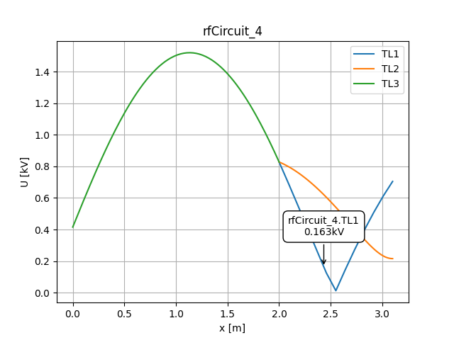
maxV, where, VSWs = ct.maxV(f=55e6, E={'TL3.E': 1})
plotVSWs(VSWs)
plt.show()
Here various steps happened in creating the circuit, let’s explain them one by one:
rfTRL makes a radio frequency Transmission Line (TL) object, it can be given various arguments:
L is the length of the TL section
OD is the outer diameter
ID is the inner diameter
Z0TL is the characteristic impedance
Zbase is the reference impedance of the S-matrix representing the TL section
dx is the dimensional step along the TL used to solve the telegraphist’s ODE.
As can be seen in the definition of TRL1, we create a conical TL by specifying an inner diameter at the leftmost side of 0.1 and an inner diameter at the rightmost side of 0.13.
rfRLC can build the following circuit structure:
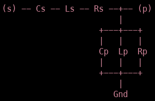
With the connecting ports being (s) and (p), the kwargs are:
Zbase : reference impedance [50 Ohm]
ports : port names [[‘s’,’p’]]
Rp : parallel resistance [+inf Ohm]
Lp : parallel inductance [+inf H]
Cp : parallel capacity [0 F]
Rs : series resistance [0 Ohm]
Ls : series inductance [0 H]
Cs : series capacity [+inf F]
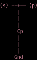
Here we only implement a parallel capacitor, i.e:
Now that we have our building blocks, it’s time to put them together in a circuit. To do this we create a rfCircuit() instance which we’ll call ct and add the blocks.
The first block which we’ll add is TRL1 which we’ll call ‘TL1’, we’ll label the leftmost port ‘T’ and the rightmost port ‘E’. As a reference point we’ll use the length of TRL3. Now we’ll do analogous additions of the other transmission lines and of the capacitor. then we’ll connect both TRL2 and TRL3 to the same input port ‘T’ and output port ‘E’ (note that we have specified the ports of TRL3 already in the block itself).
Now we’ll add our T-section containing the parallel capacitor, we labeled the source (s) as “E” and the output (p) as “oc”. Afterwards we place this circuit part 1.1m away from the place where we put our transmission lines.
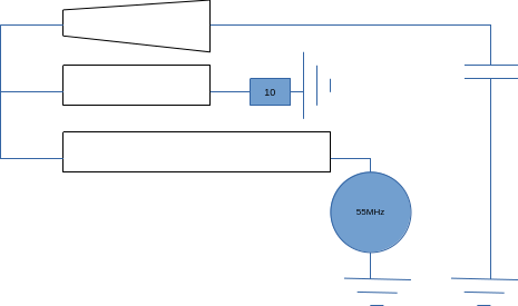
These ports now need to be connected, we first connect all the ports labeled “T” and then all the ports labeled “E”. We then proceed to leave the circuit open at the righthand side (Y=0 means zero admittance at oc) and place a 10 Ohm impedance at E, terminating the circuit there.
In the end, our circuit thus looks like:
Now we apply a signal to the point ‘TL3.E’ with a frequency of 55MHz, using maxV we can then get back maxV, which is the maximal voltage over the full circuit, where, which says where this happened and VSWs (Voltage Standing Waves) which is an array-like value containing data on how the voltage changes over the distance, this can then be plotted using plotVSWs. Note that this sets this software apart from other RF-circuitry applications such as cuqs where you may only know what happens at certain nodes, not over the whole circuit.
Running the program should show the window shown below, giving a clear insight in how the voltage changes over the circuit.