Touchstone files

To incorporate touchstone files in a circuit we can make use of the rfObject class. We’ll showcase this capability using the TOMAS ICRH matching circuit, of which a diagram is shown below

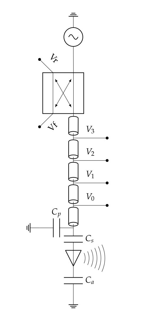
I.e the RF power source goes to a differential coupler, the output then goes through a coaxial cable containing 4 voltage probes. After this the signal goes through a capacitor L-section or the “matching box”. Then it goes through the antenna and finally to the “pre-matching capacitor” Ca.

We have the touchstone file for the antenna, called “tomas_icrh_linear_2017-vacuum.s2p”, using this we can construct the following code to create the circuit:

def Circuit(CaVal=150*1e-12,CpVal=47.94*1e-12,CsVal=133*1e-12):

     from pyRFtk import rfCircuit, rfTRL, rfRLC, rfObject, rfCoupler

     TRLStoV3 = rfTRL(L=0.235, OD=0.041, ID=0.017, dx=500)
     TRLV3toV2 = rfTRL(L=0.66, OD=0.041, ID=0.017, dx=500)
     TRLV2toV1 = rfTRL(L=0.795, OD=0.041, ID=0.017, dx=500)
     TRLV1toV0 = rfTRL(L=0.66, OD=0.041, ID=0.017, dx=500)
     TRLV0toM = rfTRL(L=0.235, OD=0.041, ID=0.017, dx=500)
     #load S matrix of antenna
     Antenna = rfObject(touchstone='tomas_icrh_linear_2017-vacuum.s2p')
     RLCLeft = rfRLC(Cs=CsVal,Cp=CpVal)
     CaRight = rfRLC(Cs=CaVal)

     ct = rfCircuit(Id="TOMAS_ICRH")

     ct.addblock('StoV3',TRLStoV3,ports=['S','V3'],relpos=0)
     ct.addblock('V3toV2',TRLV3toV2,ports=['V3','V2'],relpos=TRLStoV3.L)
     ct.addblock('V2toV1',TRLV2toV1,ports=['V2','V1'],relpos=TRLStoV3.L + TRLV3toV2.L)
     ct.addblock('V1toV0',TRLV1toV0,ports=['V1','V0'],relpos=TRLStoV3.L + TRLV3toV2.L + TRLV2toV1.L)
     ct.addblock('V0toM',TRLV0toM,ports=['V0','M'],relpos=TRLStoV3.L + TRLV3toV2.L + TRLV2toV1.L + TRLV1toV0.L)

     EndOfLine =TRLStoV3.L + TRLV3toV2.L + TRLV2toV1.L + TRLV1toV0.L + TRLV0toM.L

     ct.addblock('Matching',RLCLeft,ports=['F','G'])
     ct.addblock('Antenna',Antenna,ports=['G','H'])
     ct.addblock('RLoss',rfRLC(Rs=1),ports=['in','out'])
     ct.addblock('PreMatch',CaRight,ports=['H','I'])

     ct.connect('StoV3.S','Source')
     ct.connect('V3toV2.V3','StoV3.V3')
     ct.connect('V3toV2.V2','V2toV1.V2')
     ct.connect('V2toV1.V1','V1toV0.V1')
     ct.connect('V1toV0.V0','V0toM.V0')
     ct.connect('V0toM.M','Matching.F')
     ct.connect('Matching.G','RLoss.in')
     ct.connect('RLoss.out','Antenna.G')
     ct.connect('Antenna.H','PreMatch.H')
     ct.terminate('PreMatch.I',Z=0) #Grounding

     return ct

We added the “RLoss” resistor as to simulate the effect of a plasma. Let’s say we want to know what voltages would be measured at the nodes V0-3 if we apply 5kW at the source at 25MHz, to find this it’s as simple as

ct = Circuit()
f = 25*1e6
Solution = ct.Solution(f, E={'Source': np.sqrt(2*50*5*1E3)}, nodes=['V0toV1','V2toV3'])
V = np.zeros(4)
V[0] = np.abs(Solution['V0toV1.V0'][0])
V[1] = np.abs(Solution['V0toV1.V1'][0])
V[2] = np.abs(Solution['V2toV3.V2'][0])
V[3] = np.abs(Solution['V2toV3.V3'][0])
print(V)

Where the argument “E” indicates what we excite and “nodes” where we measure. Note that the first element of

Solution['V0toV1.V0']

was requested, this is because the elements are as follows: V,I,Vf,Vr; This also explains why we omitted the differential coupler in the definition of the circuit: Vf and Vr can directly be obtained at the node.